
Chapter 1 - Building Abstractions with Functions (Sec1.5-1.7)
5 Control
Control statements are statements that control the flow of a program’s execution based on the results of logical comparisons.
5.1 Statements
Rather than being evaluated, statements are executed. Each statement describes some change to the interpreter state, and executing a statement applies that change.
Expressions can also be executed as statements, in which case they are evaluated, but their value is discarded. Executing a pure function has no effect, but executing a non-pure function can cause effects as a consequence of function application.
5.2 Compound Statements
In general, Python code is a sequence of statements. A simple statement is a single line that doesn’t end in a colon(冒号).
Compound statements typically span multiple lines and start with a one-line header ending in a colon, which identifies the type of statement. Together, a header and an indented suite of statements is called a clause. A compound statement consists of one or more clauses.
We can understand the statements we have already introduced in these terms.
- Expressions, return statements, and assignment statements are simple statements.
- A def statement is a compound statement. The suite that follows the def header defines the function body.
5.3 Defining Functions Ⅱ: Local Assignment
In fact, functions can define a sequence of operations that extends beyond a single expression.
A return statement redirects control: the process of function application terminates whenever the first return statement is executed, and the value of the return expression is the returned value of the function being applied.
The effect of an assignment statement is to bind a name to a value in the first frame of the current environment. As a consequence, assignment statements within a function body cannot affect the global frame.
1 | def pd(x, y): |
5.4 Conditional Statements
A conditional statement in Python consists of a series of headers and suites: a required if clause, an optional sequence of elif clauses, and finally an optional else clause.
1 | if <expression>: |
The computational process of executing a conditional clause follows.
- Evaluate the header’s expression.
- If it is a true value, execute the suite. Then, skip over all subsequent clauses in the conditional statement.
Logical expressions have corresponding evaluation procedures.
这里要注意short-circuiting
To evaluate the expression <left> and <right>:
- Evaluate the subexpression <left>.
- If the result is a false value
v, then the expression evaluates tov. - Otherwise, the expression evaluates to the value of the subexpression <right>.
To evaluate the expression <left> or <right>:
- Evaluate the subexpression <left>.
- If the result is a true value
v, then the expression evaluates tov. - Otherwise, the expression evaluates to the value of the subexpression <right>.
5.5 Iteration
In addition to selecting which statements to execute, control statements are used to express repetition.
1 | def fib(n): |
5.6 Testing
Assertions. Programmers use assert statements to verify expectations, such as the output of a function being tested. An assert statement has an expression in a boolean context, followed by a quoted line of text (single or double quotes are both fine, but be consistent) that will be displayed if the expression evaluates to a false value.
1 | assert 6==5, "no" |
When writing Python in files, rather than directly into the interpreter, tests are typically written in the same file or a neighboring file with the suffix _test.py.
Doctests. Python provides a convenient method for placing simple tests directly in the docstring of a function. The first line of a docstring should contain a one-line description of the function, followed by a blank line. A detailed description of arguments and behavior may follow. In addition, the docstring may include a sample interactive session that calls the function.
1 | def fib(n): |
To verify the doctest interactions for only a single function, we use a doctest function called run_docstring_examples. Its first argument is the function to test. The second should always be the result of the expression globals(), a built-in function that returns the global environment. The third argument is True to indicate that we would like “verbose” output: a catalog of all tests run.
When writing Python in files, all doctests in a file can be run by starting Python with the doctest command line option:
python3 -m doctest <python_source_file>
6 Higher-Order Functions
这节比较重要
Functions that manipulate functions (accept other functions as arguments or return functions as values) are called higher-order functions.
6.1 Functions as Arguments
我们先来看这三个函数
1 | def sum_naturals(n): |
They are for the most part identical, differing only in name and the function of k used to compute the term to be added.
1 | def <name>(n): |
Each of these functions is a summation of terms. As program designers, we would like our language to be powerful enough so that we can write a function that expresses the concept of summation itself rather than only functions that compute particular sums.
We can do so readily in Python by taking the common template shown above and transforming the “slots” into formal parameters.
1 | ''' |
6.2 Functions as General Methods
计算golden ratio,用online python tutor试一试
1 | def improve(update, close, guess=1): |
This example illustrates two related big ideas in computer science.
- Naming and functions allow us to abstract away a vast amount of complexity. While each function definition has been trivial, the computational process set in motion by our evaluation procedure is quite intricate.
- It is only by virtue of(因为) the fact that we have an extremely general evaluation procedure for the Python language that small components can be composed into complex processes.
6.3 Defining Functions Ⅲ: Nested Definitions
我们想计算一个数a的平方根,可以这样逼近
1 | def average(x, y): |
但是,improve里的update函数只能接受一个参数
1 | def sqrt(a): |
Like local assignment, local def statements only affect the current local frame. These functions are only in scope while sqrt is being evaluated. Consistent with our evaluation procedure, these local def statements don’t even get evaluated until sqrt is called.
这里有个小点,第一次写的时候写成adder在f2里被evaluate,这是错误的,evaluate仅仅是求值,函数被调用时才会创建新的frame
例如c=add(1,2)
- 求值operator,这个时候是对add进行evaluate,看看当前frame里这个名字绑定的对象
- 求值operands
- 调用函数add,创建一个frame
对于一个user-defined function,我们总结一下
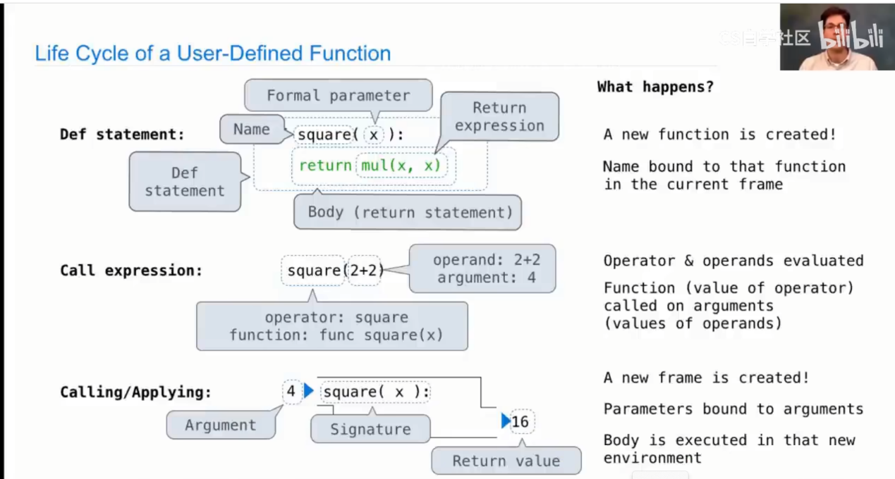
We require two extensions to our environment model to enable lexical scoping.
- Each user-defined function has a parent environment: the environment in which it was defined.
- When a user-defined function is called, its local frame extends its parent environment.
1 | def average(x, y): |
在调用sqrt(256)时,environment第一次加入sqrt的local frame,并执行 sqrt_update和sqrt_close的def语句
Function values each have a new annotation(注解) that we will include in environment diagrams from now on, a parent. The parent of a function value is the first frame of the environment in which that function was defined. Functions without parent annotations were defined in the global environment. When a user-defined function is called, the frame created has the same parent as that function.
Hence, we realize two key advantages of lexical scoping in Python.
- The names of a local function do not interfere with names external to the function in which it is defined, because the local function name will be bound in the current local environment in which it was defined, rather than the global environment.(在上个例子中,我们可以在global frame里定义
a=2019,这完全不会影响sqrt内部的函数找a,它们在f1(sqrt的frame)里找到a=256后就会停下了) - A local function can access the environment of the enclosing function, because the body of the local function is evaluated in an environment that extends the evaluation environment in which it was defined.
The sqrt_update function carries with it some data: the value for a referenced in the environment in which it was defined. Because they “enclose” information in this way, locally defined functions are often called closures(闭包).
6.4 Functions as Returned Values
The environment diagram for this example shows how the names f and g are resolved correctly, even in the presence of conflicting names.
1 | def square(x): |
6.5 Example: Newtonw’s Method
Newton’s method is a classic iterative approach to finding the arguments of a mathematical function that yield a return value of 0. These values are called the zeros(零点) of the function.
我们可以用牛顿法求平方根,事实上,求平方根并不是一件理所当然的事
牛顿法是一个迭代的算法,它对于可微函数的零点进行猜测,然后不断改进。在当前的点作切线,切线与轴的交点为,重复操作,会收敛到方程的根
其中
1 | def newton_update(f, df): |
下面我们来计算n次方根
1 | def power(x, n): |
牛顿法的初值选择比较重要,需要接近零点,否则可能不收敛。牛顿法是很重要的,至于它在计算机科学领域的应用,目前我也不大看得懂。
6.6 Currying
We can use higher-order functions to convert a function that takes multiple arguments into a chain of functions that each take a single argument. This transformation is called currying.
1 | def curried_pow(x): |
Actually, we can define functions to automate currying, as well as the inverse uncurrying transformation:
1 | def curry2(f): |
6.7 Lambda Expressions
In Python, we can create function values on the fly using lambda expressions, which evaluate to unnamed functions. A lambda expression evaluates to a function that has a single return expression as its body. Assignment and control statements are not allowed.
1 | lambda x: f(g(x)) |
The result of a lambda expression is called a lambda function. It has no intrinsic name (and so Python prints <lambda> for the name), but otherwise it behaves like any other function.
1 | s = lambda x,y : x*y |
看一下这个的environment diagram
1 | def compose1(f, g): |
In an environment diagram, the result of a lambda expression is a function as well, named with the greek letter λ (lambda).
6.8 Abstractions and First-Class Functions
We began this section with the observation that user-defined functions are a crucial abstraction mechanism, because they permit us to express general methods of computing as explicit elements in our programming language. Now we’ve seen how higher-order functions permit us to manipulate these general methods to create further abstractions.
In general, programming languages impose restrictions on the ways in which computational elements can be manipulated. Elements with the fewest restrictions are said to have first-class status. Some of the “rights and privileges” of first-class elements are:
- They may be bound to names.
- They may be passed as arguments to functions.
- They may be returned as the results of functions.
- They may be included in data structures.
Python awards functions full first-class status, and the resulting gain in expressive power is enormous.
6.9 Function Decorators
Python provides special syntax to apply higher-order functions as part of executing a def statement, called a decorator. Perhaps the most common example is a trace.
1 | def trace(fn): |
The def statement for triple has an annotation, @trace, which affects the execution rule for def. As usual, the function triple is created. However, the name triple is not bound to this function. Instead, the name triple is bound to the returned function value of calling trace on the newly defined triple function. In code, this decorator is equivalent to:
1 |
|
7 Recursive Functions
A function is called recursive if the body of the function calls the function itself, either directly or indirectly. That is, the process of executing the body of a recursive function may in turn require applying that function again.
1 | def sum_digits(n): |
When sum_digits is called on 738:
- A local frame for
sum_digitswithnbound to 738 is created, and the body ofsum_digitsis executed in the environment that starts with that frame. - Since 738 is not less than 10, the assignment statement is executed, splitting 738 into 73 and 8.
- In the following
returnstatement,sum_digitsis called on 73, the value ofall_but_lastin the current environment. - Another local frame (Its parent is global frame, 因为在f1里evaluate sum_digits时,现在f1找这个name,没找到,在global frame里找到了,而sum_digits的parent在定义时就明确了是global frame,所以调用sum_digits时创建的f2的parent是global frame) for
sum_digitsis created, this time withnbound to 73. The body ofsum_digitsis again executed in the new environment that starts with this frame. - Since 73 is also not less than 10, 73 is split into 7 and 3 and
sum_digitsis called on 7, the value ofall_but_lastevaluated in this frame. - A third local frame for
sum_digitsis created, withnbound to 7. - In the environment starting with this frame, it is true that n < 10, and therefore 7 is returned.
- In the second local frame, this return value 7 is summed with 3, the value of last, to return 10.
- In the first local frame, this return value 10 is summed with 8, the value of last, to return 18.
7.1 The Anatomy of Recursive Functions
A common pattern can be found in the body of many recursive functions. The body begins with a base case, a conditional statement that defines the behavior of the function for the inputs that are simplest to process.
The base cases are then followed by one or more recursive calls. Recursive calls always have a certain character: they simplify the original problem. Recursive functions express computation by simplifying problems incrementally.
Treating a recursive call as a functional abstraction has been called a recursive leap of faith. We define a function in terms of itself, but simply trust that the simpler cases will work correctly when verifying the correctness of the function.
7.2 Mutual Recursion
When a recursive procedure is divided among two functions that call each other, the functions are said to be mutually recursive.
1 | def is_even(n): |
Mutually recursive functions can be turned into a single recursive function by breaking the abstraction boundary between the two functions.
1 | def is_even(n): |
7.3 Printing in Recursive Functions
The computational process evolved by a recursive function can often be visualized using calls to print.
1 | def cascade(n): |
7.4 Tree Recursion
Another common pattern of computation is called tree recursion, in which a function calls itself more than once.
A function with multiple recursive calls is said to be tree recursive because each call branches into multiple smaller calls, each of which branches into yet smaller calls, just as the branches of a tree become smaller but more numerous as they extend from the trunk.
1 | def fib(n): |
7.5 Example: Partitions
We will define a function count_partitions(n, m) that returns the number of different partitions of n using parts up to m.
Notice that all the ways of partitioning n can be divided into two groups: those that include at least one m and those that do not.
1 | def count_partitions(n, m): |