Chapter 3 - Machine-Level Representation of Programs

0 Intro

依旧开头最难啃

Computers execute machine code(机器码), sequences of bytes encoding the low-level operations that manipulate data, manage memory, read and write data on storage devices, and communicate over networks. A compiler generates machine code through a series of stages, based on the rules of the programming language, the instruction set of the target machine, and the conventions followed by the operating system. The GCC C compiler generates its output in the form of assembly code(汇编代码), a textual representation of the machine code giving the individual instructions in the program. GCC then invokes both an assembler(汇编器) and a linker(链接器) to generate the executable machine code from the assembly code. In this chapter, we will take a close look at machine code and its human-readable representation as assembly code.

When programming in a high-level language such as C, and even more so in Java, we are shielded(保护、屏蔽) from the detailed machine-level implementation of our program. In contrast, when writing programs in assembly code(as was done in the early days of computing) a programmer must specify the low-level instructions the program uses to carry out a computation. Most of the time, it is much more productive and reliable to work at the higher level of abstraction provided by a high-level language. The type checking provided by a compiler helps detect many program errors and makes sure we reference and manipulate data in consistent ways. With modern optimizing compilers, the generated code is usually at least as efficient as what a skilled assembly-language programmer would write by hand. Best of all, a program written in a high-level language can be compiled and executed on a number of different machines, whereas assembly code is highly machine specific.

Even though compilers do most of the work in generating assembly code, being able to read and understand it is an important skill for serious programmers. By invoking the compiler with appropriate command-line parameters, the compiler will generate a file showing its output in assembly-code form. By reading this code, we can understand the optimization capabilities of the compiler and analyze the underlying inefficiencies in the code.

Furthermore, there are times when the layer of abstraction provided by a high-level language hides information about the run-time behavior of a program that we need to understand. For example, when writing concurrent programs using a thread package, as covered in Chapter 12, it is important to understand how program data are shared or kept private by the different threads and precisely how and where shared data are accessed. Such information is visible at the machine-code level.

In this chapter, we will learn the details of one particular assembly language and see how C programs get compiled into this form of machine code. Reading the assembly code generated by a compiler involves a different set of skills than writing assembly code by hand. We must understand the transformations typical compilers make in converting the constructs of C into machine code. Relative to the computations expressed in the C code, optimizing compilers can rearrange execution order, eliminate unneeded computations, replace slow operations with faster ones, and even change recursive computations into iterative ones. Understanding the relation between source code and the generated assembly can often be a challenge — it’s much like putting together a puzzle having a slightly different design than the picture on the box. It is a form of reverse engineering(逆向工程) — trying to understand the process by which a system was created by studying the system and working backward. In this case, the system is a machine-generated assembly language program, rather than something designed by a human. This simplifies the task of reverse engineering because the generated code follows fairly regular patterns and we can run experiments, having the compiler generate code for many different programs.

Our presentation is based on x86-64, the machine language for most of the processors found in today’s laptop and desktop machines, as well as those that power very large data centers and supercomputers. This language has evolved over a long history, starting with Intel Corporation’s first 16-bit processor in 1978, through to the expansion to 32 bits, and most recently to 64 bits. Along the way, features have been added to make better use of the available semiconductor technology, and to satisfy the demands of the marketplace. We will focus on the subset of the features used by GCC and Linux.

Our presentation focuses on the types of machine-level programs generated when compiling C and similar programming languages targeting modern operating systems.

1 A Historical Perspective

The Intel processor line, colloquially(通俗地说) referred to as x86, has followed a long evolutionary development. It started with one of the first single-chip 16-bit microprocessors, where many compromises had to be made due to the limited capabilities of integrated circuit technology at the time.

The x86 architecture has developed over many years. It began with Intel’s 8086 processor in 1978, which was a 16-bit processor. Later processors gradually added new features and improved performance. The i386 was an important step because it extended x86 to a 32-bit architecture, often called IA32. Later, x86 was extended again to 64 bits, giving us the x86-64 architecture used by most modern computers.

An important feature of x86 is backward compatibility(向后兼容). Newer processors are designed to run programs written for older processors. This makes x86 very successful, but it also makes the architecture more complicated because many old design features must still be supported. Advanced Micro Devices (AMD) also played an important role by introducing the widely adopted x86-64 extension, which was later supported by Intel. Over time, the number of transistors in processors increased dramatically, allowing processors to become much more powerful and complex.

2 Program Encodings

Suppose we write a C program as two files p1.c and p2.c. We can then compile this code using a Unix command line:

1	gcc -Og -o p p1.c p2.c

The command gcc indicates the GCC C compiler. Since this is the default compiler on Linux, we could also invoke it as simply cc. The command-line option -Og instructs the compiler to apply a level of optimization that yields machine code that follows the overall structure of the original C code. (This optimization level was introduced in GCC version 4.8. Earlier versions of GCC, as well as non-GNU compilers, will not recognize this option. For these, using optimization level one (specified with the command-line flag -O1) is probably the best choice for generating code that follows the original program structure.)

Invoking higher levels of optimization can generate code that is so heavily transformed that the relationship between the generated machine code and the original source code is difficult to understand. We will therefore use -Og optimization as a learning tool and then see what happens as we increase the level of optimization. In practice, higher levels of optimization (e.g., specified with the option -O1 or -O2) are considered a better choice in terms of the resulting program performance.

The gcc command invokes an entire sequence of programs to turn the source code into executable code. First, the C preprocessor expands the source code to include any files specified with #include commands and to expand any macros, specified with #define declarations. Second, the compiler generates assembly code versions of the two source files having names p1.s and p2.s. Next, the assembler converts the assembly code into binary object-code files p1.o and p2.o. Object code is one form of machine code — it contains binary representations of all of the instructions, but the addresses of global values are not yet filled in. Finally, the linker merges these two object-code files along with code implementing library functions (e.g., printf) and generates the final executable code file p (as specified by the command-line directive -o p). Executable code is the second form of machine code we will consider — it is the exact form of code that is executed by the processor.

2.1 Machine-Level Code

As described before, computer systems employ several different forms of abstraction, hiding details of an implementation through the use of a simpler abstract model. Two of these are especially important for machine-level programming.

First, the format and behavior of a machine-level program is defined by the instruction set architecture(指令集架构), or ISA, defining the processor state, the format of the instructions, and the effect each of these instructions will have on the state. Most ISAs, including x86-64, describe the behavior of a program as if each instruction is executed in sequence, with one instruction completing before the next one begins. The processor hardware is far more elaborate, executing many instructions con
currently, but it employs safeguards to ensure that the overall behavior matches the sequential operation dictated by the ISA.

Second, the memory addresses used by a machine-level program are virtual addresses, providing a memory model that appears to be a very large byte array. The actual implementation of the memory system involves a combination of multiple hardware memories and operating system software.

The compiler does most of the work in the overall compilation sequence, transforming programs expressed in the relatively abstract execution model provided by C into the very elementary instructions that the processor executes. The assembly-code(汇编代码) representation is very close to machine code. Its main feature is that it is in a more readable textual format, as compared to the binary format of machine code. Being able to understand assembly code and how it relates to the original C code is a key step in understanding how computers execute programs.

The machine code for x86-64 differs greatly from the original C code. Parts of the processor state are visible that normally are hidden from the C programmer:

The program counter(程序计数器) (commonly referred to as the PC, and called %rip in x86-64) indicates the address in memory of the next instruction to be executed.
The integer register file(寄存器文件) contains 16 named locations storing 64-bit values. These registers can hold addresses (corresponding to C pointers) or integer data. Some registers are used to keep track of critical parts of the program state, while others are used to hold temporary data, such as the arguments and local variables of a procedure, as well as the value to be returned by a function.
The condition code registers hold status information about the most recently executed arithmetic or logical instruction. These are used to implement conditional changes in the control or data flow, such as is required to implement if and while statements.
A set of vector registers can each hold one or more integer or floating-point values.

Whereas C provides a model in which objects of different data types can be declared and allocated in memory, machine code views the memory as simply a large byte-addressable array. Aggregate data types in C such as arrays and structures are represented in machine code as contiguous collections of bytes.

Even for scalar data types, assembly code makes no distinctions between signed or unsigned integers, between different types of pointers, or even between pointers and integers.

The program memory contains the executable machine code for the program, some information required by the operating system, a run-time stack for managing procedure calls and returns, and blocks of memory allocated by the user (e.g., by using the malloc library function). As mentioned earlier, the program memory is addressed using virtual addresses. At any given time, only limited subranges of virtual addresses are considered valid. For example, x86-64 virtual addresses are represented by 64-bit words. In current implementations of these machines, the upper 16 bits must be set to zero, and so an address can potentially specify a byte
over a range of $2^{48}$ , or 64 terabytes. More typical programs will only have access to a few megabytes, or perhaps several gigabytes. The operating system manages this virtual address space, translating virtual addresses into the physical addresses of values in the actual processor memory.

A single machine instruction performs only a very elementary operation. For example, it might add two numbers stored in registers, transfer data between memory and a register, or conditionally branch to a new instruction address. The compiler must generate sequences of such instructions to implement program constructs such as arithmetic expression evaluation, loops, or procedure calls and returns.

2.2 Code Examples

Suppose we write a C code file mstore.c :

// 只是声明：告诉编译器“这个函数长什么样”
// 参数名可以省略
long mult2(long, long);

void mulstore(long x, long y, long *dest) {
    long t = mult2(x, y);
    *dest = t;
}

To see the assembly code generated by the C compiler, we can use -S option on the command line:

1	gcc -Og -S mstore.c

This will cause GCC to run the compiler, generating an assembly file mstore.s, and go no further. (Normally it would then invoke the assembler to generate an object-code file.)

我们可以看到汇编代码文件中mstore:下有这么几行，以.开头的都可以先忽略掉，就得到

pushq   %rbx
movq    %rdx, %rbx
call    mult2@PLT
movq    %rax, (%rbx)
popq    %rbx
ret

每一行对应一条机器指令，比如，pushq指令表示将寄存器%rbx的内容压入程序栈中，这段代码中已经除去了所有关于局部变量名或数据类型的信息。

接着我们使用-c命令行选项，GCC会编译并汇编该代码

1	gcc -Og -c mstore.c

产生目标代码文件mstore.o，它是二进制格式的，无法直接查看，1368字节的文件mstore.o中有一段14字节的序列，它的十六进制表示为

1	53 48 89 d3 e8 00 00 00 00 48 89 03 5b c3

这就是上面列出的汇编指令对应的目标代码，因此，机器执行的程序只是一个字节序列，它是对一系列指令的编码，机器对产生这些指令的源代码几乎一无所知

要查看机器代码文件的内容，一类称作**disassemblers(反汇编器)**的程序非常有用，这些程序从机器码中产生一种类似于汇编码的格式。在Linux系统中，带-d命令行标志的程序OBJDUMP (object dump)可以充当这个角色

❯ objdump -d mstore.o

mstore.o:     file format elf64-x86-64


Disassembly of section .text:

0000000000000000 <mulstore>:
   0:   f3 0f 1e fa             endbr64
   4:   53                      push   %rbx
   5:   48 89 d3                mov    %rdx,%rbx
   8:   e8 00 00 00 00          callq  d <mulstore+0xd>
   d:   48 89 03                mov    %rax,(%rbx)
  10:   5b                      pop    %rbx
  11:   c3                      retq

最左边的数字是偏移量，每组字节对应一条指令

x86-64的指令长度从1到15个字节不等，常用的指令及操作数较少的指令需要的字节数少
设计指令格式的方法是，从某个给定位置开始，可以将字节唯一地解码成机器指令，比如，只有pushq %rbx可以以字节值53开头
反汇编器只靠机器码文件中的字节序列来决定汇编码，它不会访问程序的汇编码或者源代码
反汇编器使用的指令命名规则和GCC生成的汇编代码使用的有些许差别。在上例中，它省略了很多指令结尾的q，又在call和ret指令添加了q后缀，这些后缀是大小指示符，大多数情况下这些后缀可以被省略

Generating the actual executable code requires running a linker on the set of object-code files, one of which must contain a function main. Suppose in file main.c we had the following function:

#include <stdio.h>

void mulstore(long, long, long *);

int main() {
    long d;
    mulstore(2, 3, &d);
    printf("2 * 3 --> %ld\n", d);
    return 0;
}

long mult2(long a, long b) {
    long s = a * b;
    return s;
}

Then we would generate an executable program prog as follows:

1	gcc -Og prog main.c mstore.c

The file prog has grown to 8,655 bytes, since it contains not just the machine code for the procedures we provided but also code used to start and terminate the program as well as to interact with the operating system.

We can disassemble the file prog:

1	objdump -d prog

得到的内容包含下面这段

00000000000011d5 <mulstore>:
    11d5:       f3 0f 1e fa             endbr64
    11d9:       53                      push   %rbx
    11da:       48 89 d3                mov    %rdx,%rbx
    11dd:       e8 e7 ff ff ff          callq  11c9 <mult2>
    11e2:       48 89 03                mov    %rax,(%rbx)
    11e5:       5b                      pop    %rbx
    11e6:       c3                      retq
    11e7:       66 0f 1f 84 00 00 00    nopw   0x0(%rax,%rax,1)
    11ee:       00 00

This code is almost identical to that generated by the disassembly of mstore.c. One important difference is that the addresses listed along the left are different — the linker has shifted the location of this code to a different range of addresses. A second difference is that the linker has filled in the address that the callq instruction should use in calling the function mult2 (line 4 of the disassembly). One task for the linker is to match function calls with the locations of the executable code for those functions. A final difference is that we see two additional lines of code (lines 8–9). These instructions will have no effect on the program, since they occur after the return instruction (line7). They have been inserted to grow the code for the function to 16 bytes, enabling a better placement of the next block of code in terms of memory system performance.

2.3 Notes on Formatting

In the content of mstore.s, all of the lines beginning with ‘.’ are directives to guide the assembler and linker. We can generally ignore these. On the other hand, there are no explanatory remarks about what the instructions do or how they relate to the source code.

To provide a clearer presentation of assembly code, an annotated version would appear as follows:

# void multstore(long x, long y, long *dest)
# x in %rdi, y in %rsi, dest in %rdx
multstore:
pushq %rbx          # Save %rbx
movq %rdx,          # %rbx Copy dest to %rbx
call mult2          # Call mult2(x, y)
movq %rax, (%rbx)   # Store result at *dest
popq %rbx           # Restore %rbx
ret                 # Return

In our presentation, we show assembly code in ATT format (named after AT&T, the company that operated Bell Laboratories for many years), the default format for GCC, objdump, and the other tools we will consider. Other programming tools, including those from Microsoft as well as the documentation from Intel, show assembly code in Intel format. The two formats differ in a number of ways. As an example, GCC can generate code in Intel format for the sum function using the following command line:

1	gcc-Og-S-masm=intel mstore.c

3 Data Formats

Due to its origins as a 16-bit architecture that expanded into a 32-bit one, Intel uses the term “word” to refer to a 16-bit data type. Based on this, they refer to 32 bit quantities as “double words”, and 64-bit quantities as “quad words”.

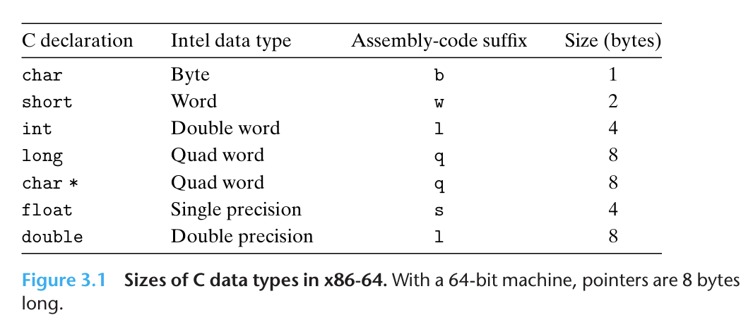
The x86-64 representations used for the primitive data types of C

标准的int值存储为双字（32位），指针存储为8字节的四字，这跟64位机器所预期的一样。本章代码示例中大部分使用指针和long数据类型，都是四字操作，x86-64指令集同样包括完整的针对字节、字和双字的指令

浮点数主要有两种形式，单精度值（4字节），对应于C语言数据类型float，双精度值对应于C语言数据类型double

大多数GCC生成的汇编代码指令都有一个字符的后缀，表明操作数的大小，比如数据传送指令有四个变种，movb, movw, movl, movq

后缀’l’表示双字因为32位也被认为是"long words"，汇编码使用’l’表示4字节整数和8字节双精度浮点数，这不会有歧义，因为浮点数使用的是一组完全不同的指令和寄存器

4 Accessing Information

An x86-64 central processing unit (CPU) contains a set of 16 general-purpose
registers(通用目的寄存器) storing 64-bit values. These registers are used to store integer data as well as pointers. Their names all begin with %r, but otherwise follow multiple different naming conventions, owing to the historical evolution of the instruction set.

The original 8086 hadeight 16-bit registers, shown in Figure 3.2 as registers %ax through %bp. Each had a specific purpose, and hence they were given names that reflected how they were to be used. With the extension to IA32, these registers were expanded to 32-bit registers, labeled %eax through %ebp. In the extension to x86-64, the original eight registers were expanded to 64 bits, labeled %rax through %rbp. In addition, eight new registers were added, and these were given labels according to a new naming convention: %r8 through %r15.

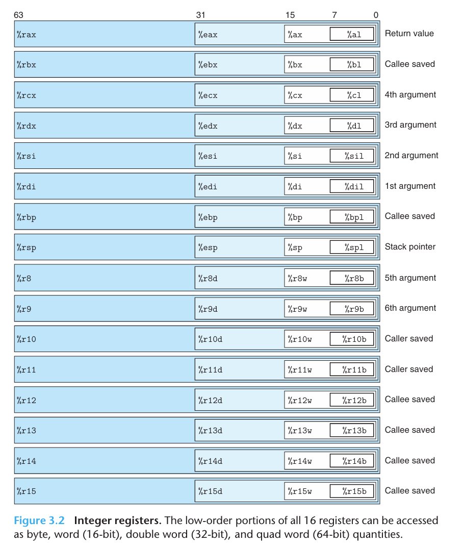
Instructions can operate on data of different sizes stored in the low-order bytes of the 16 registers. Byte-level operations can access the least significant byte, 16-bit operations can access the least significant 2 bytes, 32-bit operations can access the least significant 4 bytes, and 64-bit operations can access entire registers.

In later sections, we will present a number of instructions for copying and generating 1-, 2-, 4-, and 8-byte values. When these instructions have registers as destinations, two conventions arise for what happens to the remaining bytes in the register for instructions that generate less than 8 bytes: Those that generate 1 or 2-byte quantities leave the remaining bytes unchanged. Those that generate 4 byte quantities set the upper 4 bytes of the register to zero. The latter convention was adopted as part of the expansion from IA32 to x86-64.

As the annotations along the right-hand side of Figure 3.2 indicate, different registers serve different roles in typical programs. Most unique among them is the stack pointer, %rsp, used to indicate the end position in the run-time stack. Some instructions specifically read and write this register. The other 15 registers have more flexibility in their uses. A small number of instructions make specific use of certain registers. More importantly, a set of standard programming conventions governs how the registers are to be used for managing the stack, passing function arguments, returning values from functions, and storing local and temporary data. We’ll cover these conventions later.

4.1 Operand Specifiers

Most instructions have one or more operands(操作数) specifying the source values to use in performing an operation and the destination location into which to place the result. x86-64 supports a number of operand forms (see Figure 3.3). Source values can be given as constants or read from registers or memory. Results can be stored in either registers or memory. Thus, the different operand possibilities can be classified into three types.

The first type, immediate(立即数), is for constant values. In ATT format assembly code, these are written with a ‘$’ followed by an integer using standard C notation — for example, $-577 or $0x1F. Different instructions allow different ranges of immediate values; the assembler will automatically select the most compact(紧凑的) way of encoding a value.

The second type, register(寄存器), denotes the contents of a register, one of the sixteen 8-, 4-, 2-, or 1-byte low-order portions of the registers for operands having 64, 32, 16, or 8 bits, respectively. In Figure 3.3, we use the notation $r_a$ to denote an arbitrary register $a$ and indicate its value with
the reference $R[r_a]$ , viewing the set of registers as an array $R$ indexed by register identifiers.

The third type of operand is a memory reference(内存引用), in which we access some memory location according to a computed address, often called the effective address(有效地址). Since we view the memory as a large array of bytes, we use the notation $M_b[Addr]$ to denote a reference to the b-byte value stored in memory starting at address $Addr$ . To simplify things, we will generally drop the subscript b.

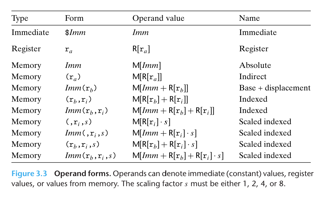
As Figure 3.3 shows, there are many different addressing modes(寻址模式) allowing different forms of memory references. The most general form is shown at the bottom of the table with syntax $Imm(r_b,r_i,s)$ . Such a reference has four components: an immediate offset $Imm$ , a base register $r_b$ , an index register $r_i$ , and a scale factor $s$ , where $s$ must be 1, 2, 4, or 8. Both the base and index must be 64-bit registers.

The effective address is computed as $Imm + R[r_b]+R[r_i]\times s$ . This general form is often seen when referencing elements of arrays. The other forms are simply special cases of this general form where some of the components are omitted.

Problem 1

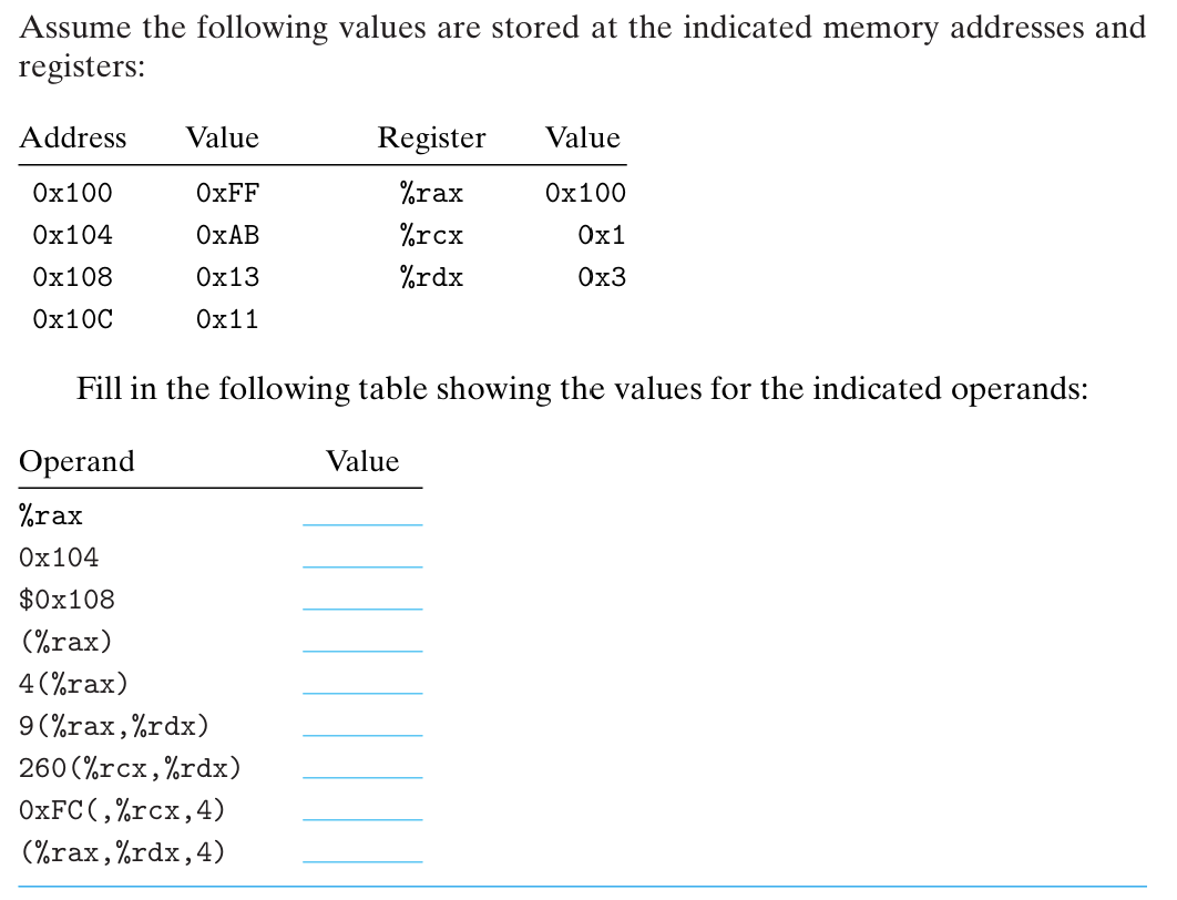
%rax是个寄存器，所以值就是里面存的值，即0x100
0x104是一个绝对地址(见图3.3 Absolute)，值就是里面存的东西，即0xAB
这是个立即数，值就是0x108
这是内存引用类型的，是指把括号内的值（即寄存器%rax存的值）作为地址，再访问这个地址里存的值，即访问地址0x100存的值，即0xFF
上一问基础上，地址偏移4位，即0x104地址存的值，即0xAB
9 + 0x100 + 0x3得到0x10C，值为0x11
260 + 0x1 + 0x3得到0x108，即0x13
0xFC + 0x1 * 4得到0x100，值为0xFF
0x100 + 0x3 * 4得到0x10C，值为0x11

4.2 Data Movement Instructions

Among the most heavily used instructions are those that copy data from one location to another. The generality of the operand notation allows a simple data movement instruction to express a range of possibilities that in many machines would require a number of different instructions. We present a number of different data movement instructions, differing in their source and destination types, what conversions they perform, and other side effects they may have. In our presentation, we group the many different instructions into instruction classes, where the instructions in a class perform the same operation but with different operand
sizes.

Figure 3.4 lists the simplest form of data movement instructions — mov class.
These instructions copy data from a source location to a destination location, without any transformation.

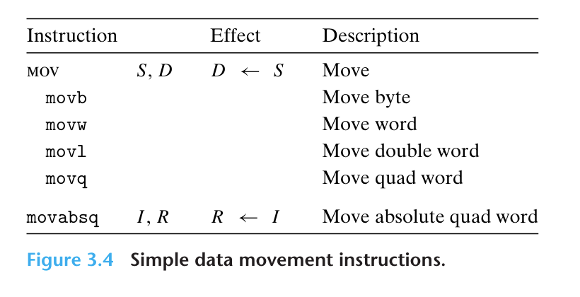
源操作数(S)指定的值是一个立即数，存储在寄存器中或者内存中，目的操作数指定一个位置，要么是一个寄存器要么是一个内存地址，x86-64限制传送指令的两个操作数不能都是内存位置，将一个值从内存位置复制到另一个内存位置需要两个指令，第一条将源值加载到寄存器中，第二条将该寄存器值写入目的位置

Referring to Figure3.2, register operands for these instructions can be the labeled portions of any of the 16 registers, where the size of the register must match the size designated by the last character of the instruction. For most cases, the mov instructions will only update the specific register bytes or memory locations indicated by the destination operand. The only exception is that when movl has a register as the destination, it will also set the high-order 4 bytes of the register to 0. This exception arises from the convention, adopted in x86-64, that any instruction that generates a 32-bit value for a register also sets the high-order portion of the register to 0.

The following mov instruction examples show the five possible combinations of source and destination types.

movl $0x4050, %eax        # Immediate--Register, 4 bytes
movw %bp, %sp             # Register--Register, 2 bytes
movb (%rdi,%rcx), %al     # Memory--Register, 1 byte
movb $-17, (%esp)         # Immediate--Memory, 1 byte
movq %rax, -12(%rbp)      # Register--Memory, 8 bytes

图3.4中最后一条指令是处理64位立即数数据的，常规的movq只能以表示为3位补码数字的立即数作为源操作数，然后把这个值符号扩展到64位的值放到目的位置，movabsq指令能够以任意64位立即数值作为源操作数，只能以寄存器作为目的

下面两类数据移动指令是在将较小的源值复制到较大的目的时使用的，所有这些指令都把数据从源(在寄存器或内存中)复制到目的寄存器，MOVZ是零扩展而MOVS是符号扩展，每条指令最后两个字符，第一个指定源的大小，第二个指定目的的大小

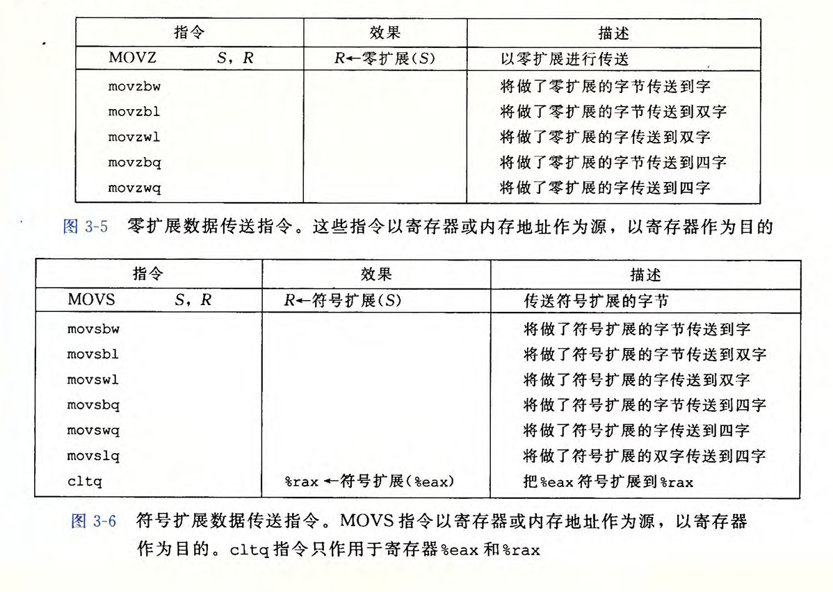
注意图3.5中没有movzlq，因为可以用以寄存器为目的的movl指令实现

As described, there are two different conventions regarding whether and how data movement instructions modify the upper bytes of a destination register. This distinction is illustrated by the following code sequence.

movabsq $0x0011223344556677, %rax   # %rax=0011223344556677
movb $-1, %al                       # %rax=00112233445566FF
movw $-1, %ax                       # %rax=001122334455FFFF
movl $-1, %eax                      # %rax=00000000FFFFFFFF
movq $-1, %rax                      # %rax=FFFFFFFFFFFFFFFF

The following example illustrates how different data movement instructions either do or donot change the high-order bytes of the destination. Observe that the three byte-movement instructions movb, movsbq, and movzbq differ from each other in subtle ways.

movabsq $0x0011223344556677, %rax   # %rax = 0011223344556677
movb $0xAA, %dl                     # %dl = AA
movb %dl, %al                       # %rax = 00112233445566AA
movsbq %dl, %rax                    # %rax = FFFFFFFFFFFFFFAA
movzbq %dl, %rax                    # %rax = 00000000000000AA

4.3 Data Movement Example

long exchange(long *xp, long y) {
    long x = *xp;
    *xp = y;
    return x;
}

得到汇编代码(下面为节选)

1
2
3

movq    (%rdi), %rax  # Get x at xp. Set as return value.
movq    %rsi, (%rdi)  # Store y at xp.
ret                   # Return.

We’ll cover the details of function call and return later. Until then, it suffices to say that arguments are passed to functions in registers. A function returns a value by storing it in register %rax, or in one of the low-order portions of this register.

When the procedure begins execution, procedure parameters xp and y are stored in registers %rdi and %rsi, respectively. Instruction 1 then reads x from memory and stores the value in register %rax, a direct implementation of the operation x = *xp in the C program. Later, register %rax will be used to return a value from the function, and so the return value will be x. Instruction 2 writes y to the memory location designated by xp in register %rdi, a direct implementation
of the operation *xp = y. This example illustrates how the mov instructions can be used to read from memory to a register (line 1), and to write from a register to memory (line 2).

Two features about this assembly code are worth noting. First, we see that what we call “pointers” in C are simply addresses. Dereferencing a pointer involves copying that pointer into a register, and then using this register in a memory reference. Second,local variables such as x are often kept in registers rather than stored in memory locations. Register access is much faster than memory access.

Problem 2

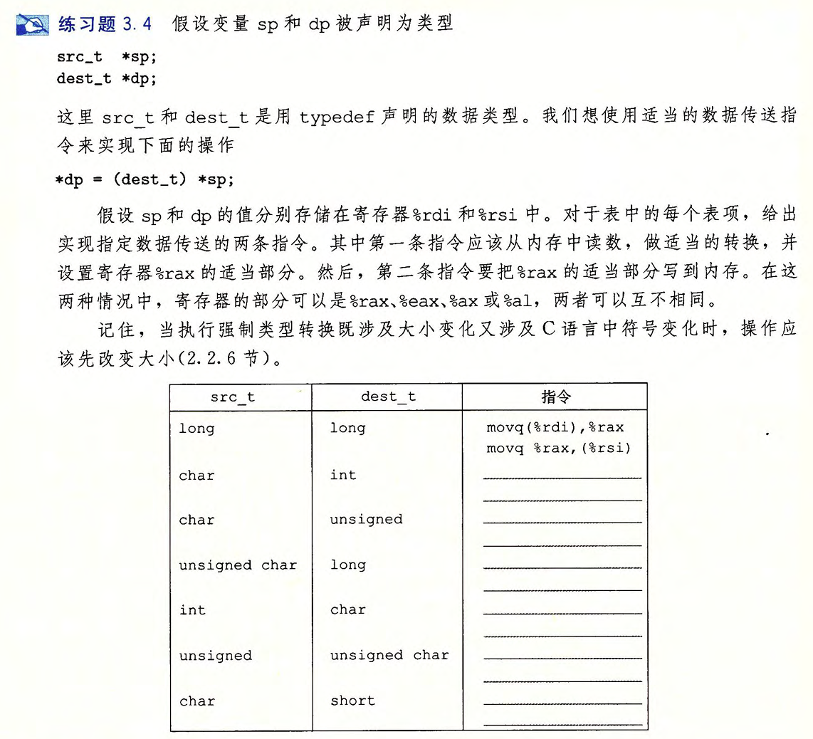
第1空，我们先写详细点

1
2
3

char *sp;
int *dp;
*dp = (int) *sp;

这里的char我们认为是signed char，在这个基础上，要先符号扩展，即

1 2	movsbl (%rdi), %eax movl %eax, (%rsi)

第一行从 %rdi 指向的内存中读取 1 字节，也就是 *sp，将其进行符号扩展得到 32 位值，然后写入 %eax (这里由于目的是寄存器，高32位会清零)
第二行将 %eax 中的 32 位值写入 %rsi 指向的内存位置，也就是写入 *dp (注意这里目的是内存，高32位并不会清零，而是保持不变)

第二空其实没区别，只不过改大小后再按无符号数去理解，但是在bit的层级上都是一样的，所以依旧写入低32位即可

1 2	movsbl (%rdi), %eax movl %eax, (%rsi)

第三空

1 2	movzbq (%rdi), %rax movq %rax, (%rsi)

书上利用了写入寄存器的低32位自动清零的性质，也可以

1 2	movzbl (%rdi), %eax movq %rax, (%rsi)

第四空，大转小直接截断

1 2	movb (%rdi), %al movb %al, (%rsi)

不过这个有点取巧，而且只适合小端机器(虽然x86-64本身就是针对小端机器的)，书上的答案会更自然，先把int完整存到寄存器再取低8位

1 2	movl (%rdi), %eax movb %al, (%rsi)

第五空

1 2	movl (%rdi), %eax movb %al, (%rsi)

第六空

1 2	movsbw (%rdi), %ax movw %ax, (%rsi)

Problem 3
已知函数

1	void decode1(long xp, long yp, long *zp);

编译后，它的汇编代码是

decode1:
    movq (%rdi), %r8
    movq (%rsi), %rcx
    movq (%rdx), %rax
    movq %r8, (%rsi)
    movq %rcx, (%rdx)
    movq %rax, (%rdi)
    ret

三个参数分别存在寄存器%rdi, %rsi, %rdx，试写出C代码

void decode1(long *xp, long *yp, long *zp) {
    long x = *xp;
    long y = *yp;
    long z = *zp;

    *yp = x;
    *zp = y;
    *xp = z;
}

4.4 Pushing and Poping Stack Data

The final two data movement operations are used to push data onto and pop data from the program stack, as documented in Figure 3.8. As we will see, the stack plays a vital role in the handling of procedure calls. By way of background, a stack is a data structure where values can be added or deleted, but only according to a “last-in, first-out” discipline. We add data to a stack via a push operation and remove it via a pop operation, with the property that the value popped will always be the value that was most recently pushed and is still on the stack. A stack can be implemented as an array, where we always insert and remove elements from one end of the array. This end is called the top of the stack.

With x86-64, the program stack is stored in some region of memory. As illustrated in Figure 3.9, the stack grows downward such that the top element of the stack has the lowest address of all stack elements. (By convention, we draw stacks upside down, with the stack “top” shown at the bottom of the figure.) The stack pointer %rsp holds the address of the top stack element.

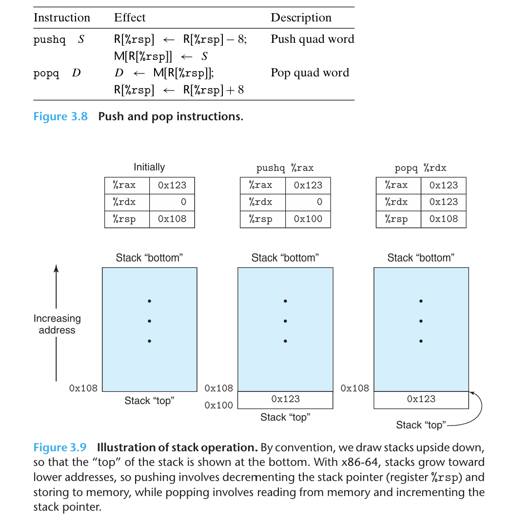
The pushq instruction provides the ability to push data onto the stack, while the popq instruction pops it. Each of these instructions takes a single operand — the data source for pushing and the data destination for popping. Pushing a quad word value onto the stack involves first decrementing(减少) the stack pointer by 8 and then writing the value at the new top-of-stack address. Therefore, the behavior of the instruction pushq %rbp is equivalent to that of the pair of instruction:

1 2	subq $8, %rsp # Decrement stack pointer movq %rbp,(%rsp) # Store %rbp on stack

except that the pushq instruction is encoded in the machine code as a single byte, whereas the pair of instructions shown above requires a total of 8 bytes. The first two columns in Figure 3.9 illustrate the effect of executing the instruction pushq %rax when %rsp is 0x108 and %rax is 0x123. First %rsp is decremented by 8, giving 0x100, and then 0x123 is stored at memory address 0x100.

Popping a quad word involves reading from the top-of-stack location and then incrementing the stack pointer by 8. Therefore, the instruction popq %rax is equivalent to the following pair of instructions:

1 2	movq (%rsp), %rax # Read %rax from stack addq $8, %rsp # Increment stack pointer

The third column of Figure3.9 illustrates the effect of executing the instruction popq %edx immediately after executing the pushq. Value 0x123 is read from memory and written to register %rdx. Register %rsp is incremented back to 0x108. As shown in the figure, the value 0x123 remains at memory location 0x104 until it is overwritten (e.g., by another push operation). However, the stack top is always considered to be the address indicated by %rsp. Since the stack is contained in the same memory as the program code and other forms of program data, programs can access arbitrary positions within the stack using the standard memory addressing methods. For example, assuming the topmost element of the stack is a quad word, the instruction movq 8(%rsp),%rdx will copy the second quad word from the stack to register %rdx

5 Arithmetic and Logical Operations

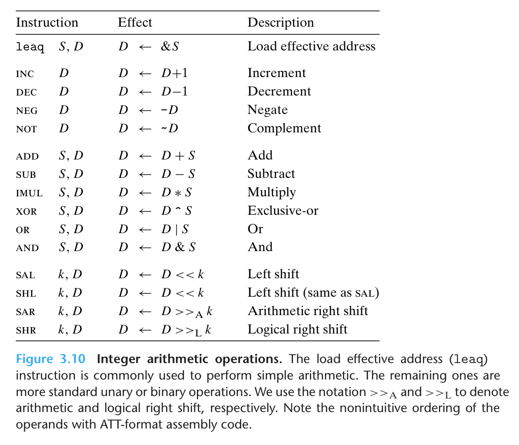
Figure 3.10 lists some of the x86-64 integer and logic operations. Most of the operations are given as instruction classes, as they can have different variants with different operand sizes. (Only leaq has no other size variants.) For example, the instruction class ADD consists of four addition instructions: addb, addw, addl, and
addq, adding bytes, words, double words, and quad words, respectively.

Indeed, each of the instruction classes shown has instructions for operating on these four different sizes of data. The operations are divided into four groups: load effective address, unary, binary, and shifts. Binary operations have two operands, while unary operations have one operand. These operands are specified using the same notation as described in Section 3.4.

5.1 Load Effective Address

The load effective address instruction(加载有效地址) leaq is actually a variant of the movq instruction. It has the form of an instruction that reads from memory to a register, but it does not reference memory at all. Its first operand appears to be a memory reference, but instead of reading from the designated location, the instruction copies the effective address to the destination. We indicate this computation in Figure 3.10 using the C address operator &S. This instruction can be used to generate pointers for later memory references. In addition, it can be used to compactly describe common arithmetic operations. For example, if register %rdx contains value x, then the instruction leaq 7(%rdx,%rdx,4), %rax will set register %rax to 5x+7. Compilers often find clever uses of leaq that have nothing to do with effective address computations. The destination operand must be a register.

long scale(long x, long y, long z) {
    long t = x + 4 * y + 12 * z;
    return t;
}

编译后

# x in %rdi, y in %rsi, z in %rdx
leaq (%rdi, %rsi, 4), %rax # x + 4 * y
leaq (%rdx, %rdx, 2), %rdx # z + 2 * z
leaq (%rax, %rdx, 4), %rax

5.2 Unary and Binary Operations

Operations in the second group are unary operations, with the single operand serving as both source and destination. This operand can be either a register or a memory location. For example, the instruction incq (%rsp) causes the 8-byte element on the top of the stack to be incremented.

The third group consists of binary operations, where the second operand is used as both a source and a destination. This syntax is reminiscent of the C assignment operators, such as x-=y. Observe, however, that the source operand is given first and the destination second. This looks peculiar for noncommutative operations. For example, the instruction subq %rax,%rdx decrements register %rdx by the value in %rax. (It helps to read the instruction as “Subtract %rax from %rdx.”) The first operand can be either an immediate value, a register, or a memory location. The second can be either a register or a memory location. As with the
mov instructions, the two operands cannot both be memory locations. Note that when the second operand is a memory location, the processor must read the value from memory, perform the operation, and then write the result back to memory.

5.3 Shift Operations

移位操作先给出移位量，第二项给出要移位的数，移位量可以是个立即数(0~255)，或者放在单字节寄存器%cl中，1个字节的移位量使得移位量的编码范围可以达到255

x86-64中，移位操作对 $w$ 位长的数据值进行操作，移位量由%cl寄存器的低 $m$ 位决定，其中 $2^m = w$ ，高位会被忽略。比如%cl的十六进制为0xFF时，salb会移7位，salw会移15位

例如假设%rax = 0x123456789ABCDEF0

1	salw $4, %ax

最终得到%rax = 0x123456789ABCEF00

移位操作的目的操作数可以是一个寄存器或是一个内存位置

5.4 Discussion

大多数算术/逻辑指令并不区分signed和unsigned，比如addq，CPU其实不在乎我们用无符号还是补码去理解bit pattern，我们用之前学到的补码、无符号数的加法规则得到结果即可

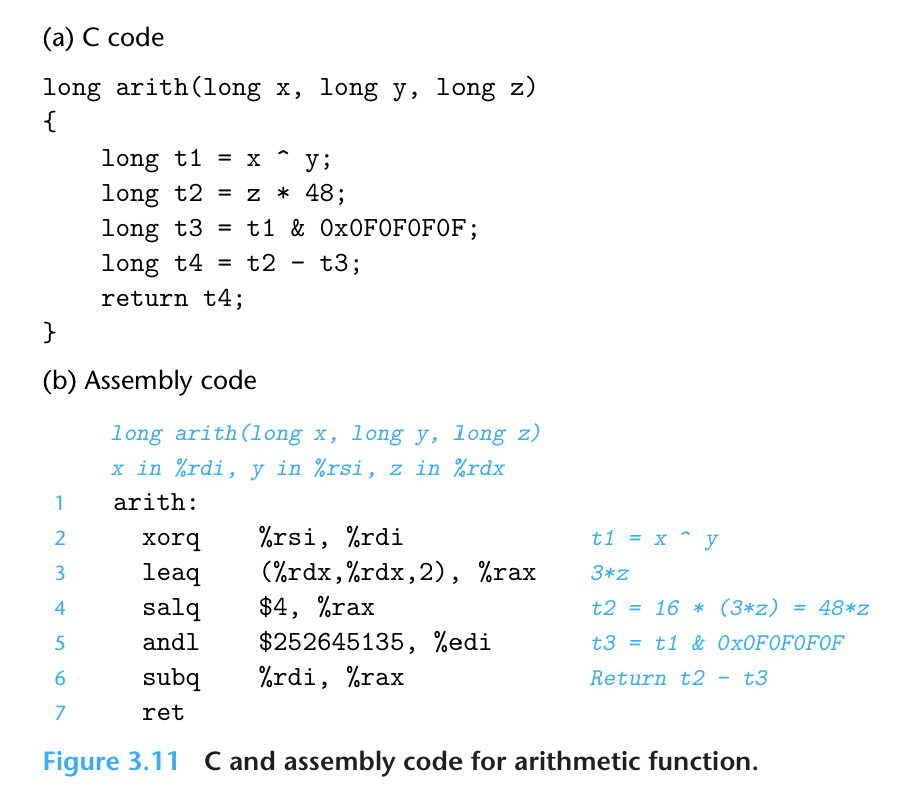
可以看到，%rax中的值先后对应于3*z, z*48和t4作为返回值，通常，编译器产生的代码中会用一个寄存器存放多个程序值，还会在寄存器间传送程序值

5.5 Special Arithmetic Operations

第二章中我们提到过，两个64位的操作数做乘法，需要128位来保留结果，而我们一般是只保留低64位

Intel把16字节的数称为八字(oct word)，图3.12描述的是支持产生两个64位数字的全128位乘积以及整数除法的指令

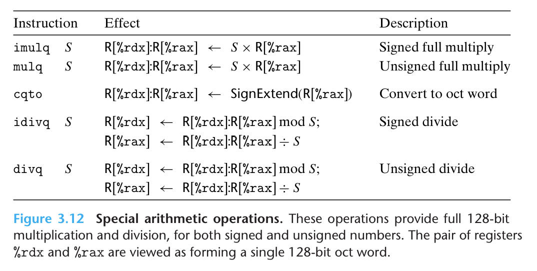
imulq指令有两种形式，图3.10中的是从两个64位操作数产生一个64位乘积，这实现了2.3.4和2.3.5中的 $*^u_{64}$ 和 $*^t_{64}$

而图3.12中的mulq和imulq两条指令可以计算两个64位值的全128位乘积，它们都要求一个参数要存在%rax中，另一个作为指令的源操作数给出，然后乘积存放在寄存器%rdx(高64位)和%rax(低64位)中

#include <inttypes.h>

typedef unsigned __int128 uint128_t;

void store_uprod(uint128_t *dest, uint64_t x, uint64_t y) {
    *dest = x * (uint128_t)y;
}

In this program, weexplicitly declare x and y to be 64-bit numbers, using definitions declared in the file inttypes.h , as part of an extension of the C standard.
Unfortunately, this standard does not make provisions for 128-bit values. Instead, we rely on support provided by GCC for 128-bit integers, declared using the name __int128. Our code uses a typedef declaration to define data type uint128_t, following the naming pattern for other data types found in inttypes.h. The code specifies that the resulting product should be stored at the 16 bytes designated by pointer dest.
编译后

# dest in %rdi, x in %rsi, y in %rdx
movq    %rsi, %rax
mulq    %rdx
movq    %rax, (%rdi)    # Store lower 8 bytes at dest
movq    %rdx, 8(%rdi)   # Store upper 8 bytes at dest+8
ret

Observe that storing the product requires two movq instructions: one for the low-order 8 bytes (line 4), and one for the high-order 8 bytes (line 5). Since the
code is generated for a little-endian machine, the high-order bytes are stored at higher addresses, as indicated by the address specification 8(%rdi).

对于除法

1 2	idivq S divq S

这里被除数是%rdx : %rax，是一个128位数，除数是S
指令把商存到%rax，把余数存到%rdx

对大多数64位除法应用，被除数也常常是一个64位的值，这个值存放在%rax中，%rdx的位应该设置为全0(无符号运算)或者%rax的符号位(有符号运算)，后者可以用cqto来完成，该指令从%rax读出符号位并复制到%rdx所有位

void remdiv(long x, long y, long *qp, long *rp) {
    long q = x / y;
    long r = x % y;
    *qp = q;
    *rp = r;
}

编译后得到

# x in %rdi, y in %rsi, qp in %rdx, rp in %rcx
movq    %rdi, %rax      # Move x to lower 8 bytes of dividend
movq    %rdx, %r8       # Copy qp
cqto                    # Sign extend to upper 8 bytes of dividend
idivq   %rsi            # Divide by y
movq    %rax, (%r8)     # Store quotient at qp
movq    %rdx, (%rcx)    # Store remainder at rp
ret

In this code, argument rp must first be saved in a different register (line 3), since argument register %rdx is required for the division operation. Lines 2, 4 then prepare the dividend by copying and sign-extending x. Following the division, the
quotient in register %rax gets stored at qp (line 6), while the remainder in register %rdx gets stored at rp (line 7).
Unsigned division makes use of the divq instruction. Typically, register %rdx is set to zero beforehand(提前).

6 Control

So far, we have only considered the behavior of straight-line code, where instructions follow one another in sequence. Some constructs in C, such as conditionals, loops, and switches, require conditional execution, where the sequence of operations that get performed depends on the outcomes of tests applied to the data. Machine code provides two basic low-level mechanisms for implementing conditional behavior: it tests data values and then alters either the control flow or the data flow based on the results of these tests.

Data-dependent control flow is the more general and more common approach for implementing conditional behavior, and so we will examine this first. Normally both statements in C and instructions in machine code are executed sequentially, in the order they appear in the program. The execution order of a set of machine code instructions can be altered with a jump instruction, indicating that control should pass to some other part of the program, possibly contingent(依情况而定的) on the result of some test. The compiler must generate instruction sequences that build upon this low-level mechanism to implement the control constructs of C.

6.1 Condition Codes

In addition to the integer registers, the CPU maintains a set of single-bit condition code(条件码) registers describing attributes of the most recent arithmetic or logical operation. These registers can then be tested to perform conditional branches. These condition codes are the most useful:

CF: Carry flag. The most recent operation generated a carry our of the most significant bit. Used to detect overflow for unsigned operations.
ZF: Zero flag. The most recent operation yielded zero.
SF: Sign flag. The most recent operation yielded a negative value.
OF: Overflow flag. The most recent operation caused a two’s-complement overflow - either negative or positive.

For example, suppose we used one of the add instructions to perform the equivalent of the C assignment t = a + b, where variables a, b, and t are integers. Then the condition codes would be set according to the following C expressions:

(unsigned) t < (unsigned) a             // CF: Unsigned overflow.
t == 0                                  // ZF: Zero.
t < 0                                   // SF: Negative.
(a < 0 == b < 0) && (t < 0 != a < 0)    // OF: Signed overflow.

leaq指令不改变任何条件码，因为它是用来进行地址计算的。除此之外，图3.10列出的所有指令都会设置条件码，对于逻辑操作，例如XOR，进位标志和溢出标志设置为0，对于移位操作，进位标志将设置为最后一个被移出的位，而溢出标志设置为0；INC和DEC指令会设置溢出和零标志，但不会改变进位标志

下面我们介绍两种指令，它们只设置条件码而不改变任何其他寄存器

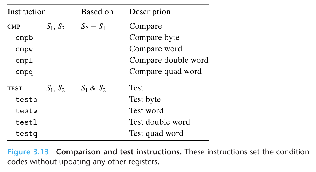
CMP指令和SUB指令的行为一样，TEST指令的行为和AND一样，除了它们只设置条件码而不改变目的寄存器的值，比如，让两个操作数是一样的，testq %rax, %rax就可以检查%rax是负数、正数还是0，看SF, ZF即可

6.2 Accessing the Condition Codes

条件码通常不会直接读取，常用的使用方法有

可以根据条件码的某种组合，将一个字节设置为0或者1
可以条件跳转到程序的某个其他的部分
可以有条件地传送数据

对于第一种情况，我们使用一类叫做SET的指令，这些指令名字的不同后缀指明了它们所考虑的条件码的组合，比如setb表示“低于时设置(set below)”
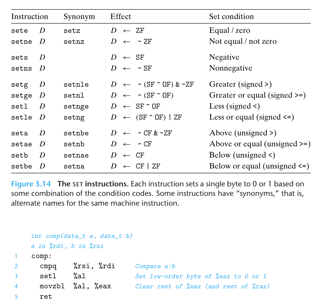
这里的set condition是假设了上一句是cmp，从而设置过了condition codes
上面的指令序列对应的是计算C语言表达式a < b，假设a, b是long类型，当没发生溢出时，SF = 1说明a - b < 0，如果溢出了，那么负溢出时a < b，这时SF = 0，所以SF ^ OF就能判断a是否小于b

某些底层的机器指令可能有多个名字，称为同义名(synonym)

对于无符号数的比较测试，执行计算t = a - b中，如果a - b < 0，CMP指令会设置进位标志为1，所以无符号比较使用的是进位标志和零标志的组合，对减法，CF = 1 表示无符号借位，也就是被减数小于减数；事实上，根据第二章的知识，我们以3位数据为例，4 - 3 = 4 + 8 - 3 = 9 = 1[001]，这时进位carry_out即第四位为1，而3 - 4 = 3 + 8 - 4 = 7 = 0[111]，carry_out = 0，所以 CF = ~carry_out

机器代码和C语言不同，它不会将每个程序值都和一个数据类型联系起来，大多数情况下，机器代码对于有符号和无符号两种情况都使用一样的指令，这是因为许多算术运算对无符号和补码算术都有一样的位级行为

6.3 Jump Instructions

Under normal execution, instructions follow each other in the order they are listed. A jump instruction can cause the execution to switch to a completely new position in the program. These jump destinations are generally indicated in assembly code by a label(标码).

考虑下面这个人造的汇编代码

  movq $0, %rax
  jmp .L1
  movq (%rax), %rdx
.L1:
  popq %rdx

The instruction jmp.L1 will cause the program to skip over the movq instruction and instead resume execution with the popq instruction. In generating the object-code file, the assembler determines the addresses of all labeled instructions and encodes the jump targets (the addresses of the destination instructions) as part of the jump instructions.

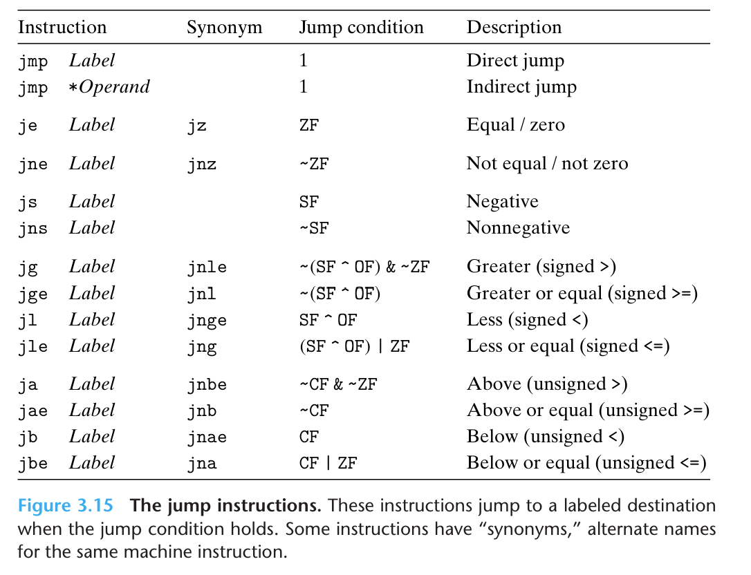
The jmp instruction jumps unconditionally. It can be either a direct jump, where the jump target is encoded
as part of the instruction, or an indirect jump, where the jump target is read from a register or a memory location.

1
2
3

jmp *%rax   # Uses the value in register %rax as the jump target

jmp *(%rax) # Reads the jump target from memory, using the value in %rax as the read address

The remaining jump instructions in the table are conditional — they either jump or continue executing at the next instruction in the code sequence, depending on some combination of the condition codes. Conditional jumps can only be direct.