4 - Asymptotics

1 An Introduction to Asymptotic Analysis

Previously, we have focused on how to save time writing the program. Now, we will learn how to make the best use of our computer’s time and memory.

We can consider the process of writing efficient programs from two different perspectives:

1. Programming Cost (everything in the course up to this date)

• How long does it take for you to develop your programs?

• How easy is it to read or modify your code?

• How maintainable is your code? (very important — much of the cost comes from maintenance (维护) and scalability (可扩展性), not development!)

2. Execution Cost (everything in the course from this point on)

• Time complexity: How much time does it take for your program to execute?

• Space complexity: How much memory does your program require?

举个例子，给定一个从小到大排序好的数组，判断里面有没有重复的元素

一个自然的想法是，把每一对元素都比较一下，更好的做法是，利用有序性，只要比较每个元素和它的下一个元素是否一样即可

2 Runtime Characterization

We want to be able to characterize (描述) the runtime of the two algorithms we previously saw. In other words, we want to come up with some proxy (指标) that communicates the overall performance of each algorithm.

/**
 * Naive Algorithm
 * Compare everything.
 */
public static boolean dup1(int[] a) {
    for (int i = 0; i < a.length; ++i) {
        for (int j = i + 1; j < a.length; ++j) {
            if (a[i] == a[j]) {
                return true;
            }
        }
    }
    return false;
}

/**
 * Better Algorithm
 * Compare only neighbors.
 */ 
public static boolean dup2(int[] a) {
    for (int i = 0; i < a.length - 1; ++i) {
        if (a[i] == a[i+1]) {
            return true;
        }
    }
    return false;
}

2.1 Technique 1

The first technique we will consider using for runtime characterization is directly measuring execution time in seconds using a client program.

• Use a physical stopwatch (not recommended).

• Use Unix’s built in time command.

• Use the Princeton Standard library which has a stopwatch class.

Using any of these methods will show that as input size increases, dup1 takes a longer time to complete, whereas dup2 completes at relatively around the same rate.

However, it could take a long time to finish running, and running times can vary by machine, compiler, input data, etc.

For these reasons, technique 1 does not meet our goals in characterizing runtimes. It’s simple, but it’s not mathematically rigorous. Moreover, the differences based on machine, compiler, input, etc. mean that the results may not clearly demonstrate the relationship between dup1 and dup2.

2.2 Technique 2A

Rather than physically timing the amount of time it takes for the algorithm to run, we can instead count the total number of operations completed by each algorithm! Intuitively, the algorithm that runs the fewer number of operations would be superior to the other. We can fix the input size N to be the same for both algorithms and compare the number of operations run.

/**
 * Naive Algorithm
 * Compare everything.
 */
public static boolean dup1(int[] a) {
    for (int i = 0; i < a.length; ++i) {
        for (int j = i + 1; j < a.length; ++j) {
            if (a[i] == a[j]) {
                return true;
            }
        }
    }
    return false;
}

Operation	Count (for N = 10000)
i = 0	1
j = i + 1	1 to 10000
<	2 to 50015001
++	0 to 50005000
==	1 to 49995000
array accesses	2 to 99990000

To summarize technique 2A, we have solved the issue of machine independence. Differences in machines do not affect the total of operations run (usually). However, it is tedious to compute all the counts for each operation. In addition, our chosen input size is arbitrary, and we do not know how much time it actually takes to run.

2.3 Technique 2B

We can resolve the issue of choosing input size by calculating the symbolic count instead, which means that we calculate our counts in terms of the input N.

Operation	Symbolic Count
i = 0	1
j = i + 1	1 to $N$
<	2 to $(N^2 + 3N + 2) / 2$
++	0 to $(N^2 + N) / 2$
==	1 to $(N^2 - N) / 2$
array accesses	2 to $N^2 - N$

Using symbolic counts allows us to see how the algorithms scales(改变大小，可译作算法在输入规模变化时如何表现) with input size. However, it is now even more tedious to calculate! It also still does not tell the actual time.

Problem
数操作的个数(表格里的数字可能跟数量差了1，忽略它即可)

/**
 * Better Algorithm
 * Compare only neighbors.
 */ 
public static boolean dup2(int[] a) {
    for (int i = 0; i < a.length - 1; ++i) {
        if (a[i] == a[i+1]) {
            return true;
        }
    }
    return false;
}

Operation	Symbolic Count
i = 0	1
++	0 to $N-1$
<	1 to $N$
==	0 to $N-1$
array accesses	2 to $2N - 2$

我们可以看到，在最坏情况下，dup2需要的操作数少于dup1，更好的说法是，随着$N$的增长，dup1最坏情况下的操作数的数量增长速度会远快于dup2

3 Asymptotic Behavior

In most applications, we are most concerned about what happens for very large values of N. This is known as the asymptotic behavior(渐进行为). We want to learn what types of algorithms are able to handle large amounts of data.

目前，我们已经把描述做到了"Clearly demonstrate the superiority of dup2 over dup1."

接下来我们做一些简化，首先，只考虑最坏情况，接着，我们只关注一种最能代表算法表现的操作，在dup1中，<, ++, ==或者array access都是可以的，我们选中的operation叫做cost model

然后，忽略低阶的项，这是因为随着$N$的增大，比如$N^3 + 100N^2 + 5N$这种式子，$N^3$会远远大于剩下的两项，甚至它们的和，所以直接忽略掉即可

最后，去掉常数系数

4 Simplified Analysis Process

Our simplified analysis process will consist of:

• Choosing our cost model, which is the representative operation we want to count.

• Figuring out the order of growth for the count of our representative operation by either:

  • Making an exact count and discarding unnecessary pieces or…

  • Using intuition/inspection to determine orders of growth. This is something that comes with practice.

其实本来有点期待，61B会把复杂度分析这部分讲的如何，虽然讲的是很细致，但其实还是跟学校教的那套差不多……

int N = A.length;
for (int i = 0; i < N; i += 1)
   for (int j = i + 1; j < N; j += 1)
      if (A[i] == A[j])
         return true;
return false;

我们来分析，执行次数最多的应该是==，当然选<什么的也可以，执行了$(N-1) + (N-2) + ... + 1 = N(N-1) / 2$次，所以最坏情况下增长情况是$N^2$级别的

5 Big-Theta

Instead of saying a function has order of growth(增长阶数)xxx, we say that function belongs to $\Theta (xxx)$

In other words, it belongs to the family of functions that have that same order of growth.

For some function $R(N)$ with order of growth $f(N)$, we write that

$$R(N)\in \Theta (f(N))$$

and there exists some positive constants $k_1, k_2$ such that

$$k_1 f(N)\le R(N)\le k_2 f(N)$$

for all values $N$ greater than some $N_0$ (a very large $N$).

6 Big-O and Big-Omega

$$R(N)\in O(f(N))$$

means that there exists some positive constants $k_2$ such that

$$R(N)\le k_2 f(N)$$

for all values $N$ greater than some $N_0$ (a very large $N$).

---

$$R(N)\in \Omega (f(N))$$

means that there exists some positive constants $k_1$ such that

$$k_1 f(N)\le R(N)$$

for all values $N$ greater than some $N_0$ (a very large $N$).

总结一下，
对一个算法，我们可以把运行时间表示成 $R(N)$，其中 $N$ 是某个代表输入规模的量。

真实的 $R(N)$ 受到每种操作实际耗时的影响，因此很难精确、通用地计算。算法分析通常抽象掉机器相关的常数，只研究当 $N$ 增大时 $R(N)$ 的增长速度。

一种常见方法是选择一个代表性操作。在各个候选操作单次都是 $\Theta(1)$ 的前提下，代表性操作通常选“执行次数增长阶最高”的那个，若这个操作单次耗时为常数，并且执行次数

$$C(N)\in \Theta(f(N))$$

那么在该模型下，运行时间通常也有

$$R(N)\in \Theta(f(N))$$

这里的“常数时间”并不意味着不同操作耗时相等，而只意味着它们的耗时不会随着输入规模 $N$ 增长。

也就是说，完全有可能 ++ 会耗时 $10\text{ ns}$，而 < 只耗时 $1\text{ ns}$。假设程序中只有这两种操作，它们的执行次数分别为 $N$ 和 $N^2$，那么真实运行时间可以粗略表示为

$$R(N)=10N+N^2\text{ ns}$$

这里 $10$ 和 $1$ 都只是与机器、具体操作有关的常数系数。当我们只关心 $N$ 增大时运行时间的增长趋势时，

$$10N+N^2\in\Theta(N^2)$$

因此

$$R(N)\in\Theta(N^2)$$

虽然一次 ++ 比一次 < 慢 $10$ 倍，但 ++ 只执行 $N$ 次，而 < 执行 $N^2$ 次。当 $N$ 足够大时，$N^2$ 这一部分会主导总运行时间。

因此，渐进分析并不是假设“所有基本操作真的花费相同时间”，而是认为普通基本操作的单次耗时都是某个与 $N$ 无关的常数。例如：

$$T_{\text{++}}=c_1,\qquad T_{<}=c_2$$

其中 $c_1$ 和 $c_2$ 完全可以不同。

如果它们分别执行 $C_1(N)$ 和 $C_2(N)$ 次，那么更一般地，

$$R(N)=c_1C_1(N)+c_2C_2(N)+\cdots$$

渐进分析会忽略这些常数系数以及低阶项，只保留最终占主导地位的增长阶。

所以以前常说的“一个基本操作认为耗费一个单位时间”，其实是一种为了方便分析而采用的抽象模型，并不是说现实中每个操作真的耗费完全相同的时间。

它的目的不是求出程序究竟运行多少毫秒，而是衡量程序的计算工作量如何随着输入规模增长。

因此：

• 实际运行时间关注的是“具体跑了多久”；
• 渐进分析关注的是“当 $N$ 变大时，运行时间增长得有多快”。

例如：

$$1000N\in\Theta(N)$$

而

$$N^2\in\Theta(N^2)$$

虽然对于较小的 $N$，$1000N$ 可能比 $N^2$ 更大，但随着 $N$ 不断增大，$N^2$ 最终一定会超过 $1000N$。这正是渐进分析所希望揭示的性质。

另外，选择“代表性操作”并不是任何时候都适用。只有当这个操作本身的单次耗时是 $\Theta(1)$，并且它的执行次数能够代表程序主要工作量时，才可以直接通过它的次数推断总运行时间。

例如：

for (int i = 0; i < N; i++) {
    x++;
}

若把 x++ 看作代表性操作，它执行 $N$ 次，而每次是 $\Theta(1)$，因此

$$R(N)\in\Theta(N)$$

但如果循环中的操作本身不是常数时间：

for (int i = 0; i < N; i++) {
    list.contains(x);
}

假设 list.contains(x) 每次需要 $\Theta(N)$ 时间，那么虽然外层循环只执行 $N$ 次，总运行时间却是

$$N\cdot\Theta(N)=\Theta(N^2)$$

因此，更准确地说，渐进分析研究的是：

$$\boxed{\text{执行次数}\times\text{单次操作的渐进成本}}$$

并最终只保留随着 $N$ 增大时占主导地位的增长阶。

7 For Loops

下面我们分析一些具体的例子

求下面程序的时间复杂度

public static void printParty(int N) {
    for (int i = 1; i <= N; i = i * 2) {
        for (int j = 0; j < i; j += 1) {
            System.out.println("hello");
            int ZUG = 1 + 1;
        }
    }
}

可以选择 println 作为代表性操作。它的单次执行时间视为常数，因此只需要分析它一共执行了多少次。

外层循环中的 i 依次为

$$1,2,4,8,\ldots,2^{\lfloor \log_2N\rfloor}$$

因此 println 的总执行次数为

$$C(N) = 1+2+4+\cdots+2^{\lfloor\log_2N\rfloor}$$

这是一个等比数列，所以

$$C(N) = 2^{\lfloor\log_2N\rfloor+1}-1$$

接下来要证明它属于 $\Theta(N)$。

根据向下取整的定义：

$$\lfloor\log_2N\rfloor \le \log_2N < \lfloor\log_2N\rfloor+1$$

对三边取 $2$ 的幂，得到

$$2^{\lfloor\log_2N\rfloor} \le N < 2^{\lfloor\log_2N\rfloor+1}$$

由右边的不等式：

$$N < 2^{\lfloor\log_2N\rfloor+1}$$

两边除以 $2$：

$$\frac N2 < 2^{\lfloor\log_2N\rfloor}$$

因此

$$\frac N2 < 2^{\lfloor\log_2N\rfloor} \le N$$

再乘以 $2$：

$$N < 2^{\lfloor\log_2N\rfloor+1} \le 2N$$

而

$$C(N) = 2^{\lfloor\log_2N\rfloor+1}-1$$

所以有

$$N-1 < C(N) \le 2N-1$$

也就是说，$C(N)$ 被两个关于 $N$ 的常数倍夹住，因此

$$C(N)\in\Theta(N)$$

于是程序的运行时间也有

$$R(N)\in\Theta(N)$$

课程中给出的证明其实不是很严谨，其实这种证明我也没想到，一开始做的时候看到$2^{\lfloor\log_2N\rfloor+1}-1$就直接认为是$\Theta (N)$了，其实这样也不太严格

8 Recursion

public static int f3(int n) {
    if (n <= 1) {
        return 1;
    }
    return f3(n-1) + f3(n-1);
}

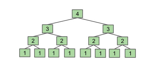
以调用f3(4)为例，它会先去算两遍f3(3)，f3(3)同理，可以发现，每次调用f3时，它自己做的工作耗时是常数，f3(1)自然不用多说，对于f3(3)，它判断后只需要将f3(2)的结果相加即可，而f3(2)也是需要等执行两次f3(1)后相加即可，因此，我们只需要看f3一共调用了几次，每次它自己做的工作都是常数时间

这并不是说f3(3)就是常数时间，而是在调用f3(3)时，它自己做的工作是常数(判断、相加，不要算函数调用内部做的工作)，至于算f3(2)，那又是调用一次f3，而在调用f3(2)的过程中又调用了两次f3

譬如我们把加法什么的，只要是常数时间的东西算成“一次操作”，那么f3(3)要先算f3(2)，这又要先算f3(1) + f3(1)，f3(1)是一次操作，所以f3(1) + f3(1)是三次操作，也就是说f3(2)整体有3次操作，所以f3(3)整体就是3 + 3 + 1 = 7次操作，这跟以3为根的那棵树的节点数量是一样的，因为f3(1) + f3(1)看上去是三次，其实就是

1 (调用最基本的f3(1)) + 1 (调用最基本的f3(1)) + 1 (f3(2)自己做的判断、加法工作)

所以运行时间是$\Theta (1 + 2 + ... + 2^{N-1}) = \Theta (2^N)$

当然，我们也可以递推

$$T(N)=2T(N-1)+\Theta(1)$$

有

$$T(N) = 2^{N-1}T(1) + \left( 2^{N-2}+2^{N-3}+\cdots+2+1 \right)\Theta(1)$$

于是

$$T(N) = 2^{N-1}T(1)+\Theta(2^{N-1})$$

而$T(1) = \Theta(1)$，故$T(N) = \Theta (2^N)$

9 Binary Search

static int binarySearch(String[] sorted, String x, int lo, int hi) {
    if (lo > hi) {
        return -1;
    }
    int m = (lo + hi) / 2;
    int cmp = x.compareTo(sorted[m]);
    if (cmp < 0) {
        return binarySearch(sorted, x, lo, m - 1);
    } else if (cmp > 0) {
        return binarySearch(sorted, x, m + 1, hi);
    } else {
        return m;
    }
}

同样地，每次调用binarySearch，函数自己做的工作都是常数时间，所以只需要数调用了几次binarySearch即可

我们以8个元素为例，考虑最坏情况，
第一次：[_ _ _ * _ _ _ _]

第二次：[/ / / / _ * _ _]

第三次：[/ / / / / / * _]

第四次：[/ / / / / / / *]

然后结束。我们可以推测出，若$N=2^k$，那么调用$log_2N + 1$次

再看看7个元素
第一次：[_ _ _ * _ _ _]

第二次：[/ / / / _ * _]

第三次：[/ / / / / / *]

能推出来$N$个元素需要$\lfloor log_2N\rfloor+1$次

严格证明

hi等于lo时，这就是最后一次调用了

每调用一次，剩下的元素就是$\lfloor \frac{N}{2} \rfloor$个
比如用上面两个例子验证下
当还剩下一个元素时，再调用一次就结束

下面我们证明一下对于任意实数 $x$ 和正整数 $m$，有

$$\left\lfloor \frac{\lfloor x\rfloor}{m} \right\rfloor = \left\lfloor \frac{x}{m} \right\rfloor.$$

证明：

设

$$k=\lfloor x\rfloor.$$

根据向下取整的定义，

$$k\le x<k+1.$$

由于 $m>0$，两边同时除以 $m$，得到

$$\frac{k}{m} \le \frac{x}{m} < \frac{k+1}{m}.$$

因为 $k$ 是整数，根据带余除法，可以写成

$$k=qm+r,$$

其中

$$q\in\mathbb Z, \qquad 0\le r<m.$$

于是

$$\frac{k}{m} = q+\frac{r}{m}.$$

由于

$$0\le\frac rm<1,$$

因此

$$\left\lfloor\frac{k}{m}\right\rfloor=q.$$

另一方面，由

$$k\le x<k+1$$

以及

$$k=qm+r$$

可得

$$qm+r \le x < qm+r+1.$$

两边同时除以 $m$：

$$q+\frac rm \le \frac xm < q+\frac{r+1}{m}.$$

因为

$$0\le r<m,$$

所以

$$0\le r\le m-1,$$

从而

$$\frac{r+1}{m}\le1.$$

因此

$$q \le \frac xm < q+1.$$

根据向下取整的定义，

$$\left\lfloor\frac xm\right\rfloor=q.$$

于是

$$\left\lfloor \frac{\lfloor x\rfloor}{m} \right\rfloor = \left\lfloor \frac{k}{m} \right\rfloor = q = \left\lfloor \frac{x}{m} \right\rfloor.$$

所以

$$\boxed{ \left\lfloor \frac{\lfloor x\rfloor}{m} \right\rfloor = \left\lfloor \frac{x}{m} \right\rfloor }$$

证毕。

---

也可以猜出结果后用数学归纳法证明，之（liu）后（gei）有（du）空（zhe）再（zi）写（zheng）

设第$r$次后只剩一个元素，我们可以得到

$$\left\lfloor \frac{N}{2^r} \right\rfloor = 1$$

于是$2^r\le N < 2^{r+1}$，所以$r = \lfloor log_2N\rfloor$

所以调用$\lfloor log_2N\rfloor + 1$次

10 Merge Sort

之前我们介绍过选择排序，即在未排序的元素中选出最小的，放到未排序元素的第一个，然后一直进行下去直到所有元素都已经被排序
假设有$N$个元素，那么第一次找最小的需要遍历数组，第二次找最小的需要遍历剩下$N-1$个元素，以此类推，因此复杂度为$\Theta (N^2)$

介绍归并排序前，我们先看merge这个操作，给两个排序好的数组，合并它们，例如
[2, 3, 11, 12] 和 [4, 6, 7, 10]

每次都比较两个数组中当前最小的元素，谁小就放到最终数组里，比如第一步后，得到
[2 _ _ _ _ _ _ _]

第二步，3比4小，得到[2 3 _ _ _ _ _ _]

如果有一个数组的元素都被放到最终数组里而另一个数组还有元素，直接复制进去即可，比如会到下面这步：
[2 3 4 6 7 10 _ _]，这时把11和12复制进去即可

假设这两个已经排序好的数组一共有$N$个元素，每次都会写入一个元素到最终数组，像2，3这种在写之前要比较一次，而11，12这种是遍历还有剩余元素的数组直接写进去，每个元素耗的都是常数时间，所以merge的时间复杂度是$\Theta (N)$，或者说，写入最终数组这个操作执行的次数一定大于等于比较操作，所以选它作为representative operation，那每个元素都会被写入，所以$\Theta (N)$

static void mergeSort(int arr[], int tmpArr[], int left, int right) {
    if (left < right) {
        int mid = (left + right) / 2;
        mergeSort(arr, tmpArr, left, mid);
        mergeSort(arr, tmpArr, mid + 1, right);
        merge(arr, tmpArr, left, mid + 1, right);
    }
    return;
}

static void merge(int arr, int tmpArr[], int left, int right, int rightEnd) {
    /** 
     * Left array: arr[left] ~ arr[right - 1]
     * Right array: arr[right] ~ arr[rightEnd]
     */
    int num = right - left + 1;
    int tmpPos = left;
    int leftEnd = right - 1;
    while (left <= leftEnd && right <= rightEnd) {
        if (arr[left] <= arr[right]) {
            tmpArr[tmpPos] = arr[left];
            left++;
            tmpPos++;
        } else {
            tmpArr[tmpPos] = arr[right];
            right++;
            tmpPos++;
        }
    }

    // Copy the left array if there are elements left.
    while (left <= leftEnd) {
        tmpArr[tmpPos] = arr[left];
        left++;
        tmpPos++;
    }

    // Copy the right array if there are elements left.
    while (right <= rightEnd) {
        tmpArr[tmpPos] = arr[right];
        right++;
        tmpPos++;
    }

    // Copy tmpArr to arr.
    for (int i = 0; i < num; ++i, rightEnd--) {
        arr[rightEnd] = tmpArr[rightEnd];
    }
}

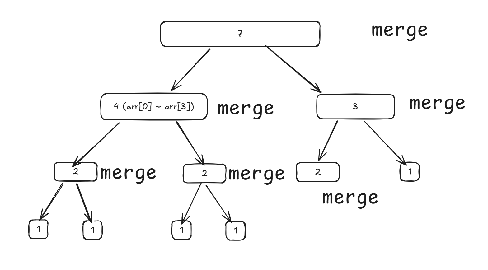
还是一样的，在每次调用mergeSort时，自己做的工作，注意这时不是常数了，自己做的工作是merge一次，所以时间是$\Theta (N)$，接下来只需要看调用了多少次mergeSort……吗？不对啊，每次merge虽然都是$\Theta (N)$，但是这个$N$也有区别，以上图为例，只有最上层的那次merge需要遍历$N=7$个元素

准确地说，第一层merge是7个元素，第二层的merge分别是4个元素和3个元素，最低层的只有一个元素的数组则是判断一下直接返回，是常数时间

如果$N=2^k$，那么这个树会很漂亮，可以得到运行时间是

$$2^k + 2\times 2^{k-1} + 4\times 2^{k-2} + ... + 2^k\times 1 = k2^k$$

如果$N$并不是刚好是2的幂次，我们也可以观察到，事实上，很多层元素之和是一样的，都是$N$，所以每一层可能会有多个数组在merge，但总共的时间，或者说写入数组这一操作的次数，或者说遍历的元素个数，都是$N$，所以我们只需要看有多少层即可，不过需要注意，如果$N$不刚好是2的幂次，那么就会出现图中这种，最底层少了一个1的情况，先算出层数为$\left\lfloor log_2N\right\rfloor + 1$，然后把总的次数夹进一个范围，即

$$N(log_2N - 1)< N\left\lfloor log_2N\right\rfloor \le C(N)\le N(\left\lfloor log_2N\right\rfloor + 1)\le Nlog_2N + 1$$

就可以得到运行时间应该是$\Theta (Nlog\ N)$

11 Summary

这篇文章写的时间比我想的要长不少，就我自己来说，对于递归的时间复杂度怎么算也是有了些更好的理解，事实上，要想严谨且准确地得出时间复杂度，我想并不是那么容易的，对我来说，如果没有严格的数学证明而只是靠感觉的话，感觉是违背了我们希望定量来分析程序的复杂度的初心了。尽管如此，若是能靠一定的直觉迅速地得到正确的复杂度，当然是更好的。